파이썬은 처음이라...Numpy
in Category / Python
Numpy
https://docs.scipy.org/doc/numpy/reference/generated/
The Basics
ndarray 는 Numpy의 배열 클래스이다.
- ndarray.ndim
- ndarray.shape
- ndarray.size
- ndarray.dtype
- ndarray.itemsize
- ndarray.data
>>> import numpy as np
>>> a = np.arange(15).reshape(3, 5)
>>> a
array([[ 0,  1,  2,  3,  4],
       [ 5,  6,  7,  8,  9],
       [10, 11, 12, 13, 14]])
>>> a.shape
(3, 5)
>>> a.ndim
2
>>> a.dtype.name
'int64'
>>> a.itemsize
8
>>> a.size
15
>>> type(a)
<type 'numpy.ndarray'>
>>> b = np.array([6, 7, 8])
>>> b
array([6, 7, 8])
>>> type(b)
<type 'numpy.ndarray'></type>
Array Creation
- 다양한 방법이 있다
- 입력한 데이터의 유형에 따라 dtype이 달라진다.
>>> import numpy as np
>>> a = np.array([2, 3, 4])
>>> a = np.array(2, 3, 4)       # ERROR
>>> b = np.array([1.2, 3.5, 5.1]) >>> a.dtype dtype('int64') >>> b.dtype dtype('float64')
>>> b = np.array([(1.5, 2, 3), (4, 5, 6)])
>>> b
array([[ 1.5,  2. ,  3. ],
       [ 4. ,  5. ,  6. ]])
배열 생성 시 dtype을 명시적으로 정할 수 있다.
>>> c = np.array( [ [1,2], [3,4] ], dtype=complex )
>>> c
array([[ 1.+0.j,  2.+0.j],
       [ 3.+0.j,  4.+0.j]])
- np.zeros()
- np.ones()
- np.empty()
기본 데이터 타입은 float64 이다.
>>> np.zeros( (3,4) )
array([[ 0.,  0.,  0.,  0.],
       [ 0.,  0.,  0.,  0.],
       [ 0.,  0.,  0.,  0.]])
>>> np.ones( (2,3,4), dtype=np.int16 )                # dtype can also be specified
array([[[ 1, 1, 1, 1],
        [ 1, 1, 1, 1],
        [ 1, 1, 1, 1]],
       [[ 1, 1, 1, 1],
        [ 1, 1, 1, 1],
        [ 1, 1, 1, 1]]], dtype=int16)
>>> np.empty( (2,3) )                                 # uninitialized, output may vary
array([[  3.73603959e-262,   6.02658058e-154,   6.55490914e-260],
       [  5.30498948e-313,   3.14673309e-307,   1.00000000e+000]])
- np.arange() : 리스트가 아닌 배열을 반환한다.
>>> np.arange( 10, 30, 5 ) array([10, 15, 20, 25]) >>> np.arange( 0, 2, 0.3 ) # it accepts float arguments array([ 0. , 0.3, 0.6, 0.9, 1.2, 1.5, 1.8]) - np.linspace() : np.arange()는 부동소수점을 사용하기 때문에 정확한 값을 예측하기 어렵다.
>>> from numpy import pi
>>> np.linspace( 0, 2, 9 )                 # 9 numbers from 0 to 2
array([ 0.  ,  0.25,  0.5 ,  0.75,  1.  ,  1.25,  1.5 ,  1.75,  2.  ])
>>> x = np.linspace( 0, 2*pi, 100 )        # useful to evaluate function at lots of points
>>> f = np.sin(x)
Pringting Arrays
- 1차원, 2차원, 3차원 배열의 출력
>>> a = np.arange(6) # 1d array >>> print(a) [0 1 2 3 4 5] >>> >>> b = np.arange(12).reshape(4,3) # 2d array >>> print(b) [[ 0 1 2] [ 3 4 5] [ 6 7 8] [ 9 10 11]] >>> >>> c = np.arange(24).reshape(2,3,4) # 3d array >>> print(c) [[[ 0 1 2 3] [ 4 5 6 7] [ 8 9 10 11]] [[12 13 14 15] [16 17 18 19] [20 21 22 23]]] - 큰 배열을 강제로 모두 출력하는 설정
>>> np.set_printoptions(threshold=np.nan)
Basic Operations
>>> a = np.array( [20,30,40,50] )
>>> b = np.arange( 4 )
>>> b
array([0, 1, 2, 3])
>>> c = a-b
>>> c
array([20, 29, 38, 47])
>>> b**2
array([0, 1, 4, 9])
>>> 10*np.sin(a)
array([ 9.12945251, -9.88031624,  7.4511316 , -2.62374854])
>>> a<35
array([ True, True, False, False])
- 행렬의 크기가 같은 배열끼리의 연산이 가능하다.
>>> A = np.array( [[1,1], ... [0,1]] ) >>> B = np.array( [[2,0], ... [3,4]] ) >>> A * B # elementwise product array([[2, 0], [0, 4]]) >>> A @ B # matrix product array([[5, 4], [3, 4]]) >>> A.dot(B) # another matrix product array([[5, 4], [3, 4]]) +=,*=로 기존 배열의 수정이 가능하다.>>> a = np.ones((2,3), dtype=int) >>> b = np.random.random((2,3)) >>> a *= 3 >>> a array([[3, 3, 3], [3, 3, 3]]) >>> b += a >>> b array([[ 3.417022 , 3.72032449, 3.00011437], [ 3.30233257, 3.14675589, 3.09233859]]) >>> a += b # b is not automatically converted to integer type Traceback (most recent call last): ... TypeError: Cannot cast ufunc add output from dtype('float64') to dtype('int64') with casting rule 'same_kind'- 데이터 타입이 다를 경우 더 일반적이거나 정확한 배열(up casting)을 따른다.
>>> a = np.ones(3, dtype=np.int32)
>>> b = np.linspace(0,pi,3)
>>> b.dtype.name
'float64'
>>> c = a+b
>>> c
array([ 1.        ,  2.57079633,  4.14159265])
>>> c.dtype.name
'float64'
>>> d = np.exp(c*1j)
>>> d
array([ 0.54030231+0.84147098j, -0.84147098+0.54030231j,
     -0.54030231-0.84147098j])
>>> d.dtype.name
'complex128'
>>> a = np.random.random((2,3))
>>> a
array([[ 0.18626021,  0.34556073,  0.39676747],
       [ 0.53881673,  0.41919451,  0.6852195 ]])
>>> a.sum()
2.5718191614547998
>>> a.min()
0.1862602113776709
>>> a.max()
0.6852195003967595
- axis를 활용하면 다양한 배열 가공이 가능하다.
>>> b = np.arange(12).reshape(3,4)
>>> b
array([[ 0,  1,  2,  3],
     [ 4,  5,  6,  7],
     [ 8,  9, 10, 11]])
>>>
>>> b.sum(axis=0)                            # sum of each column
array([12, 15, 18, 21])
>>>
>>> b.min(axis=1)                            # min of each row
array([0, 4, 8])
>>>
>>> b.cumsum(axis=1)                         # cumulative sum along each row
array([[ 0,  1,  3,  6],
     [ 4,  9, 15, 22],
     [ 8, 17, 27, 38]])
Universal Functions
- 몇 가지 수학적 기능 (범용 함수)를 제공한다.
all,any,apply_along_axis,argmax,argmin,argsort,average,bincount,ceil,clip,conj,corrcoef,cov,cross,cumprod,cumsum,diff,dot,floor,inner,inv,lexsort,max,maximum,mean,median,min,minimum,nonzero,outer,prod,re,round,sort,std,sum,trace,transpose,var,vdot,vectorize,where>>> B = np.arange(3) >>> B array([0, 1, 2]) >>> np.exp(B) array([ 1. , 2.71828183, 7.3890561 ]) >>> np.sqrt(B) array([ 0. , 1. , 1.41421356]) >>> C = np.array([2., -1., 4.]) >>> np.add(B, C) array([ 2., 0., 6.])
Indexing, Slicing and Iterating
- 1차원 배열
>>> a = np.arange(10)**3 >>> a array([ 0, 1, 8, 27, 64, 125, 216, 343, 512, 729]) >>> a[2] 8 >>> a[2:5] array([ 8, 27, 64]) >>> a[:6:2] = -1000 # equivalent to a[0:6:2] = -1000; from start to position 6, exclusive, set every 2nd element to -1000 >>> a array([-1000, 1, -1000, 27, -1000, 125, 216, 343, 512, 729]) >>> a[ : :-1] # reversed a array([ 729, 512, 343, 216, 125, -1000, 27, -1000, 1, -1000]) >>> for i in a: ... print(i**(1/3.)) ... nan 1.0 nan 3.0 nan 5.0 6.0 7.0 8.0 9.0 - 다차원 배열
>>> def f(x,y): ... return 10*x+y ... >>> b = np.fromfunction(f,(5,4),dtype=int) >>> b array([[ 0, 1, 2, 3], [10, 11, 12, 13], [20, 21, 22, 23], [30, 31, 32, 33], [40, 41, 42, 43]]) >>> b[2,3] 23 >>> b[0:5, 1] # each row in the second column of b array([ 1, 11, 21, 31, 41]) >>> b[ : ,1] # equivalent to the previous example array([ 1, 11, 21, 31, 41]) >>> b[1:3, : ] # each column in the second and third row of b array([[10, 11, 12, 13], [20, 21, 22, 23]]) >>> b[-1] # the last row. Equivalent to b[-1,:] array([40, 41, 42, 43]) .으로 다차원 배열의 인덱스를 대체할 수 있다>>> c = np.array( [[[ 0, 1, 2], # a 3D array (two stacked 2D arrays) ... [ 10, 12, 13]], ... [[100,101,102], ... [110,112,113]]]) >>> c.shape (2, 2, 3) >>> c[1,...] # same as c[1,:,:] or c[1] array([[100, 101, 102], [110, 112, 113]]) >>> c[...,2] # same as c[:,:,2] array([[ 2, 13], [102, 113]])- 기본 for 문은 첫 번째 축에 대해서 작동한다.
flat을 사용하면 각 요소에 접근이 가능하다.Indexing,Indexing(reference),newaxis,ndenumerate,indices>>> for row in b: ... print(row) ... [0 1 2 3] [10 11 12 13] [20 21 22 23] [30 31 32 33] [40 41 42 43] >>> for element in b.flat: ... print(element) ... 0 1 2 3 10 11 12 13 20 21 22 23 30 31 32 33 40 41 42 43
Shape Manipulation
Changing the shape of an array
- 배열을
shape은 변경 가능하다.>>> a = np.floor(10*np.random.random((3,4))) >>> a array([[ 2., 8., 0., 6.], [ 4., 5., 1., 1.], [ 8., 9., 3., 6.]]) >>> a.shape (3, 4) >>> a.ravel() # returns the array, flattened array([ 2., 8., 0., 6., 4., 5., 1., 1., 8., 9., 3., 6.]) >>> a.reshape(6,2) # returns the array with a modified shape array([[ 2., 8.], [ 0., 6.], [ 4., 5.], [ 1., 1.], [ 8., 9.], [ 3., 6.]]) >>> a.T # returns the array, transposed array([[ 2., 4., 8.], [ 8., 5., 9.], [ 0., 1., 3.], [ 6., 1., 6.]]) >>> a.T.shape (4, 3) reshape은 수정된 형태로 배열을 반환resize는 배열 자체를 수정>>> a array([[ 2., 8., 0., 6.], [ 4., 5., 1., 1.], [ 8., 9., 3., 6.]]) >>> a.resize((2,6)) >>> a array([[ 2., 8., 0., 6., 4., 5.], [ 1., 1., 8., 9., 3., 6.]])- -1을 사용하면 나머지 값을 자동을 계산한다.
>>> a.reshape(3,-1)
array([[ 2.,  8.,  0.,  6.],
     [ 4.,  5.,  1.,  1.],
     [ 8.,  9.,  3.,  6.]])
Stacking together different arrays
vstack과hstack으로 서로 다른 배열을 합칠 수 있다.>>> a = np.floor(10*np.random.random((2,2))) >>> a array([[ 8., 8.], [ 0., 0.]]) >>> b = np.floor(10*np.random.random((2,2))) >>> b array([[ 1., 8.], [ 0., 4.]]) >>> np.vstack((a,b)) array([[ 8., 8.], [ 0., 0.], [ 1., 8.], [ 0., 4.]]) >>> np.hstack((a,b)) array([[ 8., 8., 1., 8.], [ 0., 0., 0., 4.]])column_stack은 1차원 배열들을 2차원 배열로 반환한다.- 2차원 배열의 경우
hstack과 동일한 기능을 수행한다. row_stack은vstack과 동일한 기능을 수행한다.>>> from numpy import newaxis >>> np.column_stack((a,b)) # with 2D arrays array([[ 8., 8., 1., 8.], [ 0., 0., 0., 4.]]) >>> a = np.array([4.,2.]) >>> b = np.array([3.,8.]) >>> np.column_stack((a,b)) # returns a 2D array array([[ 4., 3.], [ 2., 8.]]) >>> np.hstack((a,b)) # the result is different array([ 4., 2., 3., 8.]) >>> a[:,newaxis] # this allows to have a 2D columns vector array([[ 4.], [ 2.]]) >>> np.column_stack((a[:,newaxis],b[:,newaxis])) array([[ 4., 3.], [ 2., 8.]]) >>> np.hstack((a[:,newaxis],b[:,newaxis])) # the result is the same array([[ 4., 3.], [ 2., 8.]])r_과c_를 이용해 배열을 만들 수 있다.>>> np.r_[1:4,0,4] array([1, 2, 3, 0, 4])
Splitting one array into several smaller ones
- 배열 분리가 가능하다.
>>> a = np.floor(10*np.random.random((2,12)))
>>> a
array([[ 9.,  5.,  6.,  3.,  6.,  8.,  0.,  7.,  9.,  7.,  2.,  7.],
     [ 1.,  4.,  9.,  2.,  2.,  1.,  0.,  6.,  2.,  2.,  4.,  0.]])
>>> np.hsplit(a,3)   # Split a into 3
[array([[ 9.,  5.,  6.,  3.],
     [ 1.,  4.,  9.,  2.]]), array([[ 6.,  8.,  0.,  7.],
     [ 2.,  1.,  0.,  6.]]), array([[ 9.,  7.,  2.,  7.],
     [ 2.,  2.,  4.,  0.]])]
>>> np.hsplit(a,(3,4))   # Split a after the third and the fourth column
[array([[ 9.,  5.,  6.],
     [ 1.,  4.,  9.]]), array([[ 3.],
     [ 2.]]), array([[ 6.,  8.,  0.,  7.,  9.,  7.,  2.,  7.],
     [ 2.,  1.,  0.,  6.,  2.,  2.,  4.,  0.]])]
Copies and Views
No Copy at All
- a 와 b는 같은 배열을 가리키고 있다.
>>> a = np.arange(12)
>>> b = a            # no new object is created
>>> b is a           # a and b are two names for the same ndarray object
True
>>> b.shape = 3,4    # changes the shape of a
>>> a.shape
(3, 4)
View or Shallow Copy
view는 새로운 배열을 만들지만 값은 공유하고 있다.>>> c = a.view() >>> c is a False >>> c.base is a # c is a view of the data owned by a True >>> c.flags.owndata False >>> >>> c.shape = 2,6 # a's shape doesn't change >>> a.shape (3, 4) >>> c[0,4] = 1234 # a's data changes >>> a array([[ 0, 1, 2, 3], [1234, 5, 6, 7], [ 8, 9, 10, 11]])- 배열을 slicing 한 경우 해당 배열의
view를 반환하기 때문에 데이터 변경 시 원본 데이터도 변경된다.>>> s = a[ : , 1:3] # spaces added for clarity; could also be written "s = a[:,1:3]" >>> s[:] = 10 # s[:] is a view of s. Note the difference between s=10 and s[:]=10 >>> a array([[ 0, 10, 10, 3], [1234, 10, 10, 7], [ 8, 10, 10, 11]])
Deep Copy
copy는 완전한 복사본을 만들며 원본 데이터를 가리키지 않는다.>>> d = a.copy() # a new array object with new data is created >>> d is a False >>> d.base is a # d doesn't share anything with a False >>> d[0,0] = 9999 >>> a array([[ 0, 10, 10, 3], [1234, 10, 10, 7], [ 8, 10, 10, 11]])- 원본 배열이 더 이상 필요하지 않는 경우 잘라낸 후
copy로 복사본을 만든다. b = a[:100]를 사용하는 경우 원본 데이터를 삭제하더라도b.base가 원본 데이터를 참조하고 있다.>>> a = np.arange(int(1e8)) >>> b = a[:100].copy() >>> del a # the memory of ``a`` can be released.
Less Basic
Broadcasting rules
Fancy indexing and index tricks
Indexing with Arrays of Indices
>>> a = np.arange(12)**2                       # the first 12 square numbers
>>> i = np.array( [ 1,1,3,8,5 ] )              # an array of indices
>>> a[i]                                       # the elements of a at the positions i
array([ 1,  1,  9, 64, 25])
>>>
>>> j = np.array( [ [ 3, 4], [ 9, 7 ] ] )      # a bidimensional array of indices
>>> a[j]                                       # the same shape as j
array([[ 9, 16],
       [81, 49]])
- 다차원 배열의 경우 1차원 인덱스 배열은 첫 번째 차원을 가리킨다.
>>> palette = np.array( [ [0,0,0], # black ... [255,0,0], # red ... [0,255,0], # green ... [0,0,255], # blue ... [255,255,255] ] ) # white >>> image = np.array( [ [ 0, 1, 2, 0 ], # each value corresponds to a color in the palette ... [ 0, 3, 4, 0 ] ] ) >>> palette[image] # the (2,4,3) color image array([[[ 0, 0, 0], [255, 0, 0], [ 0, 255, 0], [ 0, 0, 0]], [[ 0, 0, 0], [ 0, 0, 255], [255, 255, 255], [ 0, 0, 0]]]) - 배열의 크기가 같으면 다차원에 대한 인덱스 배열을 사용할 수 있다.
>>> a = np.arange(12).reshape(3,4)
>>> a
array([[ 0,  1,  2,  3],
     [ 4,  5,  6,  7],
     [ 8,  9, 10, 11]])
>>> i = np.array( [ [0,1],                        # indices for the first dim of a
...                 [1,2] ] )
>>> j = np.array( [ [2,1],                        # indices for the second dim
...                 [3,3] ] )
>>>
>>> a[i,j]                                     # i and j must have equal shape
array([[ 2,  5],
     [ 7, 11]])
>>>
>>> a[i,2]
array([[ 2,  6],
     [ 6, 10]])
>>>
>>> a[:,j]                                     # i.e., a[ : , j]
array([[[ 2,  1],
      [ 3,  3]],
     [[ 6,  5],
      [ 7,  7]],
     [[10,  9],
      [11, 11]]])
>>> l = [i,j]
>>> a[l]                                       # equivalent to a[i,j]
array([[ 2,  5],
     [ 7, 11]])
np.array([i, j])를 사용할 수 없다.>>> s = np.array( [i,j] ) >>> a[s] # not what we want Traceback (most recent call last): File "<stdin>", line 1, in ? IndexError: index (3) out of range (0<=index<=2) in dimension 0 >>> >>> a[tuple(s)] # same as a[i,j] array([[ 2, 5], [ 7, 11]])- 인덱스 배열로 각 축의 최대값을 구할 수 있다.
>>> time = np.linspace(20, 145, 5) # time scale >>> data = np.sin(np.arange(20)).reshape(5,4) # 4 time-dependent series >>> time array([ 20. , 51.25, 82.5 , 113.75, 145. ]) >>> data array([[ 0. , 0.84147098, 0.90929743, 0.14112001], [-0.7568025 , -0.95892427, -0.2794155 , 0.6569866 ], [ 0.98935825, 0.41211849, -0.54402111, -0.99999021], [-0.53657292, 0.42016704, 0.99060736, 0.65028784], [-0.28790332, -0.96139749, -0.75098725, 0.14987721]]) >>> >>> ind = data.argmax(axis=0) # index of the maxima for each series >>> ind array([2, 0, 3, 1]) >>> >>> time_max = time[ind] # times corresponding to the maxima >>> >>> data_max = data[ind, range(data.shape[1])] # => data[ind[0],0], data[ind[1],1]... >>> >>> time_max array([ 82.5 , 20. , 113.75, 51.25]) >>> data_max array([ 0.98935825, 0.84147098, 0.99060736, 0.6569866 ]) >>> >>> np.all(data_max == data.max(axis=0)) True - 값을 할당하고자 하는 대상으로 인덱스 배열을 사용할 수 있다.
>>> a = np.arange(5) >>> a array([0, 1, 2, 3, 4]) >>> a[[1,3,4]] = 0 >>> a array([0, 0, 2, 0, 0]) - 같은 곳에 여러 번 할당할 경우 마지막 값만 적용된다.
>>> a = np.arange(5)
>>> a[[0,0,2]]=[1,2,3]
>>> a
array([2, 1, 3, 3, 4])
>>> a[[0,0,2]]+=1       # 한번만 수행
>>> a
array([3, 1, 4, 3, 4])
Indexing with Boolean Arrays
- 배열과 같은 크기의 Boolean 배열을 생성할 수 있다.
>>> a = np.arange(12).reshape(3,4) >>> b = a > 4 >>> b # b is a boolean with a's shape array([[False, False, False, False], [False, True, True, True], [ True, True, True, True]]) >>> a[b] # 1d array with the selected elements array([ 5, 6, 7, 8, 9, 10, 11]) >>> a[b] = 0 # All elements of 'a' higher than 4 become 0 >>> a array([[0, 1, 2, 3], [4, 0, 0, 0], [0, 0, 0, 0]]) - 다음 코드로 이미지를 생성할 수 있다.
>>> import numpy as np
>>> import matplotlib.pyplot as plt
>>> def mandelbrot( h,w, maxit=20 ):
...     """Returns an image of the Mandelbrot fractal of size (h,w)."""
...     y,x = np.ogrid[ -1.4:1.4:h*1j, -2:0.8:w*1j ]
...     c = x+y*1j
...     z = c
...     divtime = maxit + np.zeros(z.shape, dtype=int)
...
...     for i in range(maxit):
...         z = z**2 + c
...         diverge = z*np.conj(z) > 2**2            # who is diverging
...         div_now = diverge & (divtime==maxit)  # who is diverging now
...         divtime[div_now] = i                  # note when
...         z[diverge] = 2                        # avoid diverging too much
...
...     return divtime
>>> plt.imshow(mandelbrot(400,400))
>>> plt.show()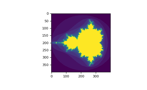
- 다차원의 배열에 대해 Boolean 배열을 이용하여 원하는 부분을 선택할 수 있다.
>>> a = np.arange(12).reshape(3,4)
>>> b1 = np.array([False,True,True])             # first dim selection
>>> b2 = np.array([True,False,True,False])       # second dim selection
>>>
>>> a[b1,:]                                   # selecting rows
array([[ 4,  5,  6,  7],
     [ 8,  9, 10, 11]])
>>>
>>> a[b1]                                     # same thing
array([[ 4,  5,  6,  7],
     [ 8,  9, 10, 11]])
>>>
>>> a[:,b2]                                   # selecting columns
array([[ 0,  2],
     [ 4,  6],
     [ 8, 10]])
>>>
>>> a[b1,b2]                                  # a weird thing to do
array([ 4, 10])
ix_()
>>> a = np.array([2,3,4,5])
>>> b = np.array([8,5,4])
>>> c = np.array([5,4,6,8,3])
>>> ax,bx,cx = np.ix_(a,b,c)
>>> ax
array([[[2]],
       [[3]],
       [[4]],
       [[5]]])
>>> bx
array([[[8],
        [5],
        [4]]])
>>> cx
array([[[5, 4, 6, 8, 3]]])
>>> ax.shape, bx.shape, cx.shape
((4, 1, 1), (1, 3, 1), (1, 1, 5))
>>> result = ax+bx*cx
>>> result
array([[[42, 34, 50, 66, 26],
        [27, 22, 32, 42, 17],
        [22, 18, 26, 34, 14]],
       [[43, 35, 51, 67, 27],
        [28, 23, 33, 43, 18],
        [23, 19, 27, 35, 15]],
       [[44, 36, 52, 68, 28],
        [29, 24, 34, 44, 19],
        [24, 20, 28, 36, 16]],
       [[45, 37, 53, 69, 29],
        [30, 25, 35, 45, 20],
        [25, 21, 29, 37, 17]]])
>>> result[3,2,4]
17
>>> a[3]+b[2]*c[4]
17
>>> def ufunc_reduce(ufct, *vectors):
...    vs = np.ix_(*vectors)
...    r = ufct.identity
...    for v in vs:
...        r = ufct(r,v)
...    return r
>>> ufunc_reduce(np.add,a,b,c)
array([[[15, 14, 16, 18, 13],
        [12, 11, 13, 15, 10],
        [11, 10, 12, 14,  9]],
       [[16, 15, 17, 19, 14],
        [13, 12, 14, 16, 11],
        [12, 11, 13, 15, 10]],
       [[17, 16, 18, 20, 15],
        [14, 13, 15, 17, 12],
        [13, 12, 14, 16, 11]],
       [[18, 17, 19, 21, 16],
        [15, 14, 16, 18, 13],
        [14, 13, 15, 17, 12]]])
Indexing with strings
Linear Algebra
선형대수학
Simple Array Operations
>>> import numpy as np
>>> a = np.array([[1.0, 2.0], [3.0, 4.0]])
>>> print(a)
[[ 1.  2.]
 [ 3.  4.]]

>>> a.transpose()
array([[ 1.,  3.],
       [ 2.,  4.]])

>>> np.linalg.inv(a)
array([[-2. ,  1. ],
       [ 1.5, -0.5]])

>>> u = np.eye(2) # unit 2x2 matrix; "eye" represents "I"
>>> u
array([[ 1.,  0.],
       [ 0.,  1.]])
>>> j = np.array([[0.0, -1.0], [1.0, 0.0]])

>>> j @ j        # matrix product
array([[-1.,  0.],
       [ 0., -1.]])

>>> np.trace(u)  # trace
2.0

>>> y = np.array([[5.], [7.]])
>>> np.linalg.solve(a, y)
array([[-3.],
       [ 4.]])

>>> np.linalg.eig(j)
(array([ 0.+1.j,  0.-1.j]), array([[ 0.70710678+0.j        ,  0.70710678-0.j        ],
       [ 0.00000000-0.70710678j,  0.00000000+0.70710678j]]))
Tricks and Tips
“Automatic” Reshaping
>>> a = np.arange(30)
>>> a.shape = 2,-1,3  # -1 means "whatever is needed"
>>> a.shape
(2, 5, 3)
>>> a
array([[[ 0,  1,  2],
        [ 3,  4,  5],
        [ 6,  7,  8],
        [ 9, 10, 11],
        [12, 13, 14]],
       [[15, 16, 17],
        [18, 19, 20],
        [21, 22, 23],
        [24, 25, 26],
        [27, 28, 29]]])
Vector Stacking
x = np.arange(0,10,2)                     # x=([0,2,4,6,8])
y = np.arange(5)                          # y=([0,1,2,3,4])
m = np.vstack([x,y])                      # m=([[0,2,4,6,8],
                                          #     [0,1,2,3,4]])
xy = np.hstack([x,y])                     # xy =([0,2,4,6,8,0,1,2,3,4])
Histograms
>>> import numpy as np
>>> import matplotlib.pyplot as plt
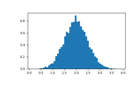
>>> # Build a vector of 10000 normal deviates with variance 0.5^2 and mean 2
>>> mu, sigma = 2, 0.5
>>> v = np.random.normal(mu,sigma,10000)
>>> # Plot a normalized histogram with 50 bins
>>> plt.hist(v, bins=50, density=1) # matplotlib version (plot)
>>> plt.show()
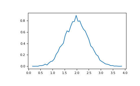
>>> # Compute the histogram with numpy and then plot it
>>> (n, bins) = np.histogram(v, bins=50, density=True)  # NumPy version (no plot)
>>> plt.plot(.5*(bins[1:]+bins[:-1]), n)
>>> plt.show()